Getting started
This page will guide you through your first PCT simulation and reconstruction. It is split into five separate steps:
Monte Carlo simulation
A proton CT set-up typically involves several elements:
a proton source
two detectors that track the position, direction and energy of incoming protons
an object through which the protons will interact
GATE is a software that allows the definition of the above-described elements, place them in space, and simulate the movements and interactions of protons in a physically realistic way. Please refer to the GATE user manual for detailed information about how to install and use GATE.
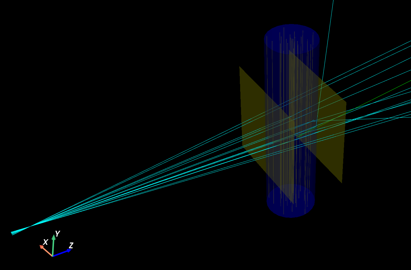
Since its version 10, GATE offers a Python interface. PCT provides an example of a proton CT simulation that can be found in gate/protonct.py. This simulation defines a 200 MeV divergent proton beam that goes through a phantom which is sandwiched between two planar detectors that track protons’ position, direction and energy. The set-up is illustrated by the picture below.
Assuming that GATE was properly installed, proton CT data can be generated with the following command:
python gate/protonct.py --output gate_simulation --verbose
The output is stored in ROOT files in the gate_simulation folder. PhaseSpaceIn.root contains the data for the upstream detector, while PhaseSpaceOut.root that of the downstream detector. protonct.txt contains details and statistics about the simulation.
You can explore additional options provided by protonct.py by running
python gate/protonct.py --help
Of course, feel free to explore the content of protonct.py directly to adapt it to your needs.
Protons pairing
In the set-up described above, protons are detected twice, first in the upstream detector, then in the downstream detector. The two resulting datasets must be merged together in a single dataset that contains both the upstream and downstream data per proton. This is known as track recontruction in the field of particle physics. PCT provides a utility that achieves this pairing: pctpairprotons.
The data can be paired using the application as follows:
python pctpairprotons.py \
    --input-in gate_simulation/PhaseSpaceIn.root \
    --input-out gate_simulation/PhaseSpaceOut.root \
    --psin PhaseSpaceIn \
    --psout PhaseSpaceOut \
    --plane-in -110 \
    --plane-out 110 \
    --output pairs.mhd \
    --verbose
The arguments are as follows:
The
--input-inand--input-outoptions correspond to the ROOT files of the upstream and downstream detectors, respectively.The
--psinand--psoutarguments are the names of the trees to read in the ROOT files.The
--plane-inand--plane-outoptions correspond to the position of the detectors along the \(z\) axis, in millimeters (in PCT, protons always travel along the \(z\) axis).The
--outputoption gives the pattern of the name of the generated files (one file per projection in our case). The outputs are MHD files that store data in the format assumed by PCT, described in this page.
As before, and for all PCT commands, you can find the list of arguments using the --help (shorthand -h) flag.
Pairs filtering
The proton pairs generated in the previous step may include protons that underwent nuclear interactions or that were incorrectly paired (in case of real data). These protons do not follow the forward model assumed by most reconstruction algorithms and should be filtered out for improving image quality (see [Schulte et al, Med. Phys., 2008]). Such protons can be filtered out according to their relative exit angle and energy. PCT provides the pctpaircuts application for this purpose.
pctpaircuts provides sensible defaults for its various options, hence the most basic usage is as follows:
pctpaircuts \
    --input pairs0000.mhd \
    --output pairs_cut0000.mhd \
    --verbose
Of course, in our case, we need to do the filtering on all the pair files that were generated in the previous step. For example, if the computer is running Bash, this can be achieved with a for loop:
for i in {0000..0719}; do
    echo "Processing pairs ${i}"
    pctpaircuts \
        --input pairs${i}.mhd \
        --output pairs_cut${i}.mhd \
        --verbose
done
Applying pair cuts is optional, but highly recommended.
Pairs binning
The next step is to bin the proton pairs in order to produce distance-driven projections, following the procedure explained in [Simon Rit et al, Med. Phys. 2013]. The corresponding PCT application is pctbinning. One projection will be generated per proton pairs file and a for loop is needed again:
for i in {0000..0719}; do
    echo "Binning pairs ${i}"
    pctbinning \
        --input pairs_cut${i}.mhd \
        --output proj${i}.mhd \
        --source -1000. \
        --size=200,1,220 \
        --spacing=2,1,1 \
        --verbose
done
The --source parameter is used to provide the source position relatively to the isocenter along the \(z\) axis. This parameter is crucial and defaults to 0, i.e., a parallel geometry. Setting a wrong source position results in malformed projections thus in an erroneous reconstruction.
The --size (in voxels) and --spacing (in millimeters) define the lattice of the projections.
Tomographic reconstruction
First, we need to generate a file that represents the geometry of our scanner. RTK provides the rtksimulatedgeometry tool that generates this file:
rtksimulatedgeometry \
    --output geometry.xml \
    --nproj 720 \
    --sid 1000 \
    --sdd 1100
--nproj corresponds to the number of projections, --sid to the source-to-isocenter distance, and --sdd to the source-to-detector distance. For more information about RTK, please refer to the RTK documentation.
Finally, the tomographic image reconstruction algorithm can be achieved using distance-driven FDK [Simon Rit et al, Med. Phys. 2013]. The corresponding PCT application is pctfdk:
pctfdk \
    --geometry geometry.xml \
    --path . \
    --regexp proj....\\.mhd \
    --output recon.mhd \
    --size=210,1,210 \
    --verbose
where --geometry is the geometry file generated above, --path is the path to the folder containing the projections, --regexp is a regular expression used to select the projection files, --output is the output file name, and --size is the size in voxels of the output image (here a 2D image, hence a size of 1 in the \(y\) direction).
The resulting image can be visualized by any MHD image viewer, such as vv.

Note that to keep the running times in this guide fast enough, not enough statistics are generated to yield a nice output image. This is just an illustration of the PCT reconstruction workflow.
PCT also provides Python functions that behave exactly like the applications described above. For illustration, the exact same simulation as the one described in this page is reimplemented in Python here.
Conclusion
This guide gives an overview of a complete workflow that uses GATE to generate proton CT data, and PCT to process the data all the way to image reconstruction. To further familiarize yourself with PCT, you can explore the other applications offered by PCT, customize the current workflow with additional parameters using the --help flag, or implement your own simulation in GATE and try to produce a reconstruction.